Excel Use Formula to Determine Which Column to Look at
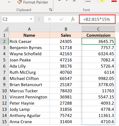
Using the VLOOKUP Formula to Lookup Value in Column and Return Value of Another Column. In case you have one column of numbers say column C that lists weekly or monthly sales you can calculate percentage change using this formula.
Excel Compare Two Columns For Matches And Differences Ablebits Com
There are two types of VLOOKUP formulas.

. Heres what this formula does. Formula LOOKUP419 A2A6 B2B6 Looks up 419 in column A and returns the value from column B that is in the same row. The formula you would enter is.
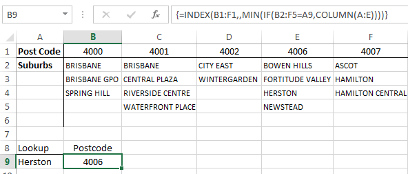
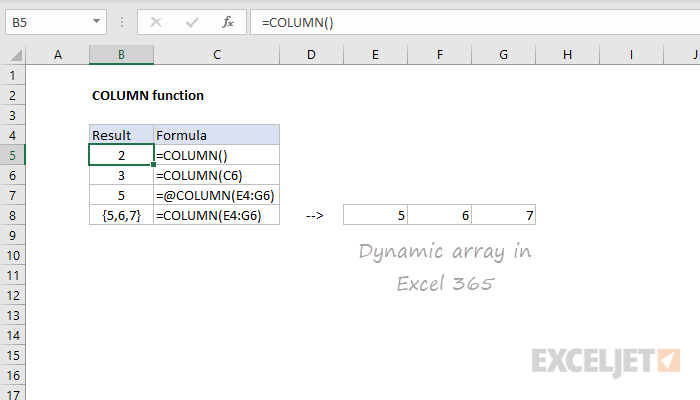
With no reference the function returns the column of the cell that contains the formula. 1 Your data needs to be set up in a table in this example the table name is Data1 2 The table needs to. The value in the Result column is the outcome of the IF formula The logical test checks to see whether the cell in the Day column B5 Wednesday we use the speech marks to tell Excel the value were performing the test on is text rather than a number If the value in the Day cell is Wednesday then the result will be Yes.
C3-C2C2 Where C2 is the 1 st and C3 is the 2 nd cell with data. Furthermore there is another similar type of formula formed using the VLOOKUP function. When I enter the Total formula the formula automatically fills the entire column.
R3 is the cell i had the time in. Orange LOOKUP575 A2A6 B2B6. Insert the formula in NOT ISERROR MATCH A2B2B10010 the formula bar.
Reference is any cell reference. To make sure all formulas are consistent I need to copy the formula down again. The plus 1 allows for excel returning midnight to 0059 as 0.
The key is this snippet. INDEXC3C13SUMPRODUCTB3B13C16D3D13C18ROWC3C130 You use the SUMPRODUCT function to find out the row where both criteria are met and return the. Heres the result youll see.
One gives the exact match of the lookup value and the other gives a partial match. IFORISNUMBERSEARCHstring1 cell ISNUMBERSEARCHstring2 cell value_to_return. Using the formula above we can get the last column that is in a range with a formula based on the COLUMN function.
INDIRECTB4 The B4 in the formula above is not a Cell reference. Heres how it looks in the Excel spreadsheet. VLOOKUPA2Data1COLUMNData1Location0 There are a few conditions.
If you ever work with large tables of data and you want to insert a VLOOKUP formula that dynamically updates to the next column as you copy it across then the VLOOKUP with the COLUMNS function is what you need. MODCOLUMNB5K5-COLUMNB51L50 Here the formula uses the COLUMN. The syntax of the COLUMN function COLUMNreference Theres only a single argument reference.
Let us first see the exact match. The new formula would look something like this. So in the formula below the first six results of the choose function are C referring to night shift then at 6am the shift changes to A day shift.
Press Enter to assign the formula to C2. Now lets look at the same formulas in an Excel table on the next sheet. Firstly enter the formula A1385 into the Cell C1 the first cell of column where you will enter the same formula secondly select the entire Column C and then click Home Fill Down.
Copy this formula into the D column. For our example the cell we want to check is A2. At this point the first formula is out of sync with the rest.
The corresponding formula in Excel is as follows. The INDIRECT function is used to convert a text string into a range for use inside another formula. You can run the function without it.
Select the output cell and use the following formula. Instead you could use a formula using a combination of SUMPRODUCT INDEX and ROW functions such as this one. I found this to be the simplest way to convert time into 3 shifts.
It is surrounded by double quotation marks so it is a text string. When you include this reference the function returns the column number of the specified cell. SUMIFSINDEXtbl_invMATCHC7tbl_invHeaders0INDEXtbl_invMATCHB7tbl_invHeaders0B8 where we use INDEXMATCH arguments for both the first sum_range argument and the second criteria_range argument.
Count rows that contain specific values In this example the goal is to count the number of rows in the data that contain the value in cell G4 which is 19. You can use the SUMIF formula in Excel to calculate percentages of a total that match criteria you specify. There is no need to copy it down.
This formula should be used if youre looking to identify cells that contain at least one of many words youre searching for. Actually there is a Fill command on Excel Ribbon to help you apply formula to an entire column or row quickly. The formula used is MINCOLUMNA3C5COLUMNSA3C5-1.
The col_index_num part of the VLOOKUP function dynamically updates as you copy it across your worksheet. As a simple example the following formula will return the value in Cell B4. If you want to apply the formula to entire row just enter the formula into the first cell.
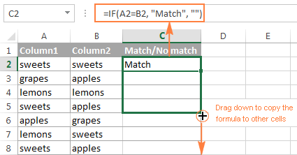
Drag the formula down to the other cells in column C clicking and dragging the little icon on the bottom-right of C2. When we give a single cell as a reference the COLUMN function will return the column number for that particular reference. You can use the COLUMN function to quickly determine the col_index_num of the VLOOKUP formula without having to count columns.
Excel will match the entries in column A with the ones in column B.
Excel Formula Vlookup With Numbers And Text Excel Formula Excel Text
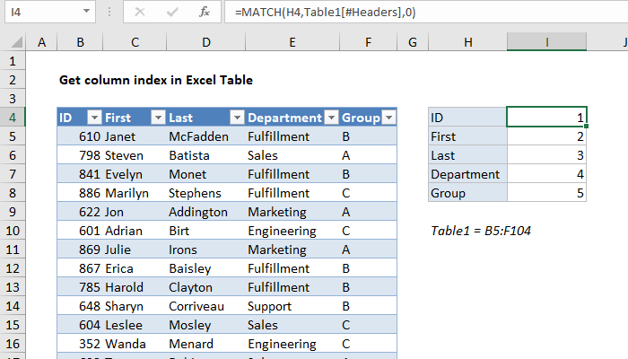
Excel Formula Get Column Index In Excel Table Exceljet
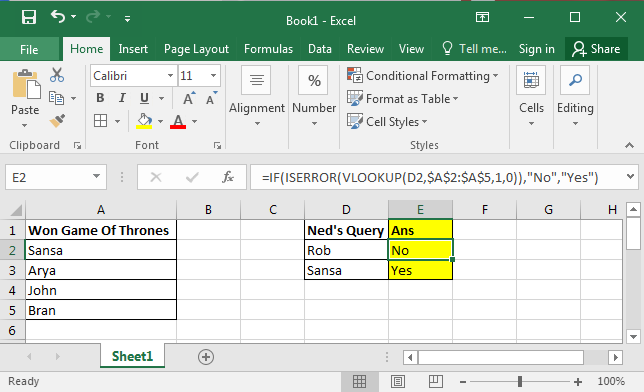
Check If A Value Exists Using Vlookup Formula
How To Apply Formula To Entire Column In Excel 5 Easy Ways Trump Excel
Excel Find Column Containing A Value My Online Training Hub
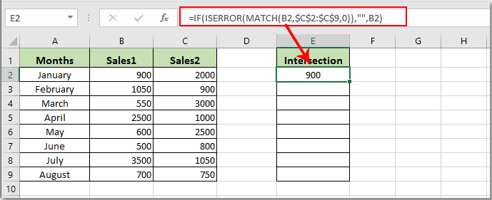
How To Find Intersection Of Two Column Lists In Excel

Excel Formula Find Longest String In Column Exceljet
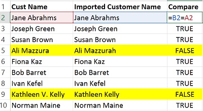
Two Ways To Compare Columns In Excel Pryor Learning

Tom S Tutorials For Excel Look Up Intersecting Value By Row And Column Criteria Tom Urtis
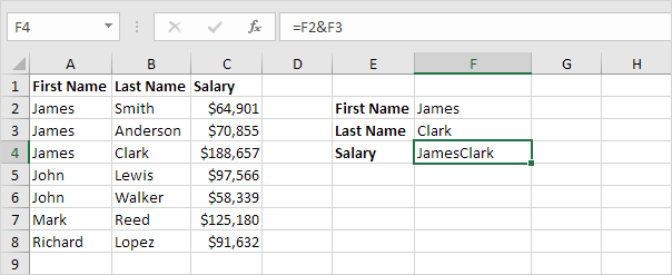
Two Column Lookup In Excel In Easy Steps
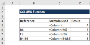
Column Function Formula Uses How To Use Column In Excel

Excel Formula Lookup Entire Column Exceljet

Index Function Excel Myexcelonline Excel Formula Excel Tutorials Microsoft Excel
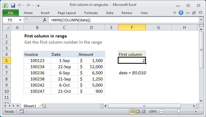
Excel Formula First Column Number In Range Exceljet
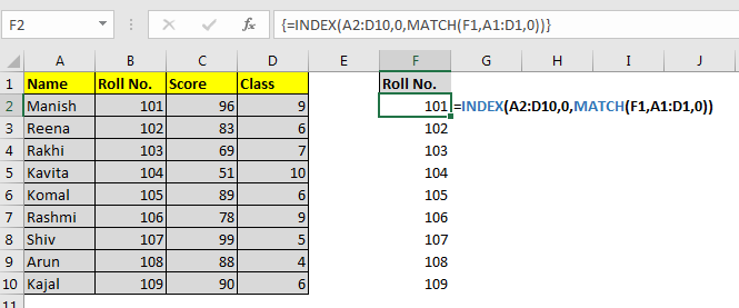
How To Lookup Entire Column In Excel Using Index Match

Autofit Columns Using Macros Myexcelonline In 2021 Excel For Beginners Microsoft Excel Formulas Excel Tutorials

Autofit Columns Using Macros Myexcelonline In 2021 Excel Tutorials Microsoft Excel Formulas Excel For Beginners
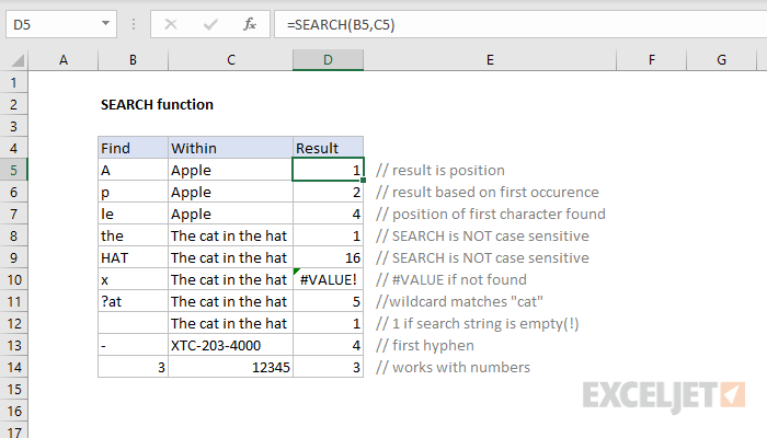
How To Use The Excel Search Function Exceljet
How To Use The Excel Column Function Exceljet


Comments
Post a Comment